Build and train deep learning models
This section covers the use of the Python API with deep learnig models. It shows how to build and train a small fully convolutional model from patches extracted in the images. The example shows how a model can be trained (1) from patches-images, or (2) from TFRecords files.
Classes and files
- fcnn_model.py implements a small fully convolutional U-Net like model,
called
FCNNModel, with the preprocessing and normalization functions that inherit fromotbtf.BaseModel - train_from_patches-images.py shows how to train the model from a list of patches-images
- train_from_tfrecords.py shows how to train the model from TFRecords files
- create_tfrecords.py shows how to convert patch-images into TFRecords files
- helper.py contains a few helping functions
Datasets
Tensorflow datasets are the most practical way to feed a network data during training steps. In particular, they are very useful to train models with data parallelism using multiple workers (i.e. multiple GPU devices). Since OTBTF 3, two kind of approaches are available to deliver the patches:
- Create TF datasets from patches-images: the first approach implemented in OTBTF, relying on geospatial raster formats supported by GDAL. Patches are stacked in rows. patches-images are friendly because they can be visualized like any other image. However this approach is not very optimized, since it generates a lot of I/O and stresses the filesystem when iterating randomly over patches.
- Create TF datasets from TFRecords files. The principle is that a number of patches are stored in TFRecords files (google protobuf serialized data). This approach provides the best performances, since it generates less I/Os since multiple patches are read simultaneously together. It is the recommended approach to work on high end gear. It requires an additional step of converting the patches-images into TFRecords files.
Patches-images based datasets
Patches-images are generated from the PatchesExtraction application of OTBTF.
They consist in extracted patches stacked in rows into geospatial rasters.
The otbtf.DatasetFromPatchesImages provides access to patches-images as a
TF dataset. It inherits from the otbtf.Dataset class, which can be a base class
to develop other raster based datasets.
The use_streaming option can be used to read the patches on-the-fly
on the filesystem. However, this can cause I/O bottleneck when one training step
is shorter that fetching one batch of data. Typically, this is very common with
small networks trained over large amount of data using multiple GPUs, causing the
filesystem read operation being the weak point (and the GPUs wait for the batches
to be ready). The class offers other functionalities, for instance changing the
iterator class with a custom one (can inherit from otbtf.dataset.IteratorBase)
which is, by default, an otbtf.dataset.RandomIterator. This could enable to
control how the patches are walked, from the multiple patches-images of the
dataset.
Suppose you have extracted some patches with the PatchesExtraction
application with 2 sources:
- Source "xs": patches images xs_1.tif, ..., xs_N.tif
- Source "labels": patches images labels_1.tif, ..., labels_N.tif
To create a dataset from this set of patches can be done with
otbtf.DatasetFromPatchesImages as shown below.
dataset = DatasetFromPatchesImages(
    filenames_dict={
        "input_xs_patches": ["xs_1.tif", ..., "xs_N.tif"],
        "labels_patches": ["labels_1.tif", ..., "labels_N.tif"]
    }
)
Getting the Tensorflow dataset is done doing:
Here the targets_keys list contains all the keys of the target tensors.
We will explain later why this has to be specified.
You can also convert the dataset into TFRecords files:
TFRecords are the subject of the next section!
TFRecords batches datasets
TFRecord based datasets are implemented in the otbtf.tfrecords module.
They basically deliver patches from the TFRecords files, which can be created
with the to_tfrecords() method of the otbtf.Dataset based classes.
Depending on the filesystem characteristics and the computational cost of one
training step, it can be good to select the number of samples per TFRecords file.
Another tweak is the shuffling: since one TFRecord file contains multiple patches,
the way TFRecords files are accessed (sometimes, we need them to be randomly
accessed), and the way patches are accessed (within a buffer, of size set with
the shuffle_buffer_size), is crucial.
Creating TFRecords based datasets is super easy:
dataset = TFRecords("/tmp")
tf_dataset = dataset.read(
    shuffle_buffer_size=1000,
    batch_size=8,
    target_keys=["predictions"]
)
Model
Overview
Let's define the setting for our model:
# Number of classes estimated by the model
N_CLASSES = 2

# Name of the input
INPUT_NAME = "input_xs"

# Name of the target output
TARGET_NAME = "predictions"

# Name (prefix) of the output we will use at inference time
OUTPUT_SOFTMAX_NAME = "predictions_softmax_tensor"
Our model estimates 2 classes. The input name is input_xs, and the target output is predictions. This target output will be used to compute the loss value, which is used ultimately to drive the learning of the network. The name of the output that we want to use at inference time is predictions_softmax_tensor. We won't use this tensor for anything else than inference.
To build our model, we can build from scratch building on tf.keras.Model,
but we will see how OTBTF helps a lot with the otbtf.BaseModel class.
First, let's take a look to this schema:
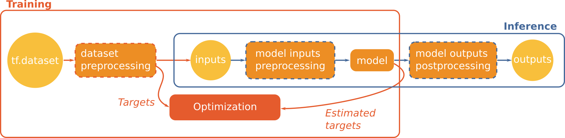
As we can see, we can distinguish two main functional blocks:
- training
- inference
Dataset transformation
During training, we need to preprocess the samples generated by the dataset to feed the network and the loss computation, that will guide how weights will be updated. This data transformation is generally required to put the data in the format expected by the model.
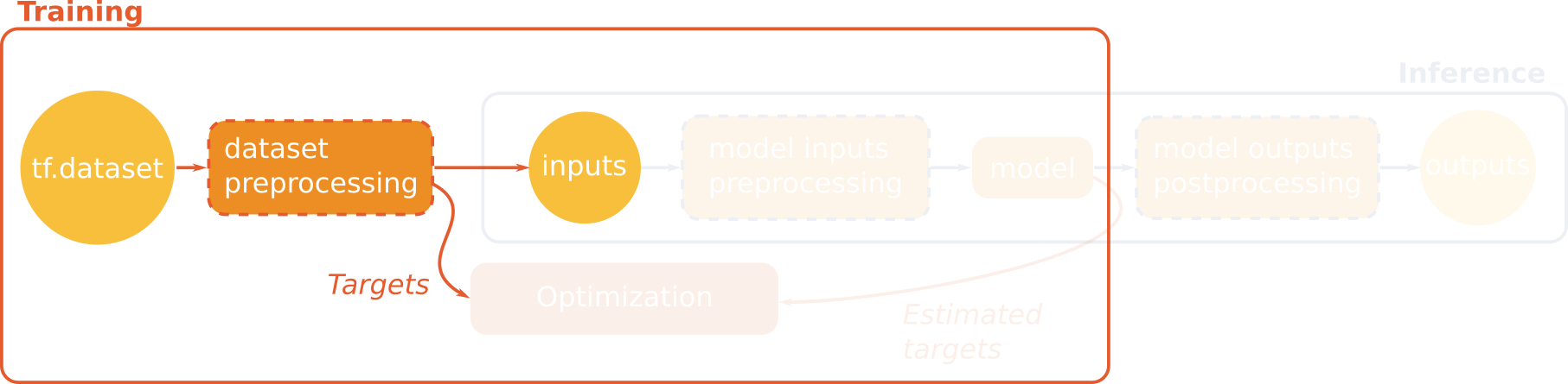
In our example, the terrain truth consists in labels which are integer values ranging from 0 to 1. However, the loss function that computes the cross entropy expects one hot encoding. The first thing to do is hence to transform the labels values into a one hot vector:
def dataset_preprocessing_fn(examples: dict):
    return {
        INPUT_NAME: examples["input_xs_patches"],
        TARGET_NAME: tf.one_hot(
            tf.squeeze(tf.cast(examples["labels_patches"], tf.int32), axis=-1),
            depth=N_CLASSES
        )
    }
As you can see, we don't modify the input tensor, since we want to use it
as it in the model.
Note that since version 4.2.0 the otbtf.ops.one_hot can ease the transform:
def dataset_preprocessing_fn(examples: dict):
    return {
        INPUT_NAME: examples["input_xs_patches"],
        TARGET_NAME: otbtf.ops.one_hot(
            labels=examples["labels_patches"],
            nb_classes=N_CLASSES
        )
}
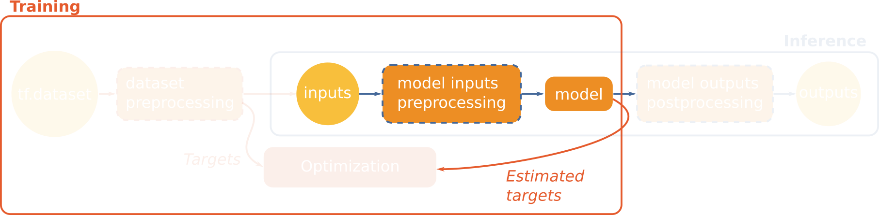
Model inputs preprocessing
The model is intended to work on real world images, which have often 16 bits signed integers as pixel values. The model has to normalize these values such as they fit the [0, 1] range before applying the convolutions. This is called normalization.
This is the purpose of normalize_inputs(), which has to be implemented as
model method. The method inputs a dictionary of tensors, and returns a
dictionary of normalized tensors. The transformation is done multiplying the
input by 0.0001, which guarantee that the 12-bits encoded Spot-7 image pixels
is in the [0, 1] range. Also, we cast the input tensor, which is originally of
type integer, to floating point.
class FCNNModel(ModelBase):
    def normalize_inputs(self, inputs: dict):
        return {INPUT_NAME: tf.cast(inputs[INPUT_NAME], tf.float32) * 0.0001}
Network implementation
Then we implement the model itself in FCNNModel.get_outputs(). The model
must return a dictionary of tensors. All keys of the target tensors must be in
the returned dictionary (in our case: the predictions tensor). These target
keys will be used later by the optimizer to perform the optimization of the
loss.
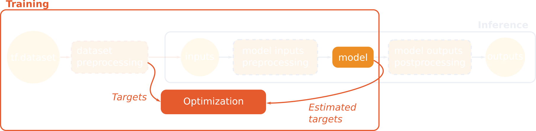
Our model is built with an encoder composed of 4 downscaling convolutional blocks, and its mirrored reversed decoder with skip connections between the layers of same scale. The last layer is a softmax layer that estimates the probability distribution for each class, and its output is used to perform the computation of the cross entropy loss with the terrain truth one hot encoded labels. Its name is predictions so that the loss crosses the terrain truth and the estimated values.
...
    def get_outputs(self, normalized_inputs: dict) -> dict:

        def _conv(inp, depth, name):
            conv_op = tf.keras.layers.Conv2D(
                filters=depth,
                kernel_size=3,
                strides=2,
                activation="relu",
                padding="same",
                name=name
            )
            return conv_op(inp)

        def _tconv(inp, depth, name, activation="relu"):
            tconv_op = tf.keras.layers.Conv2DTranspose(
                filters=depth,
                kernel_size=3,
                strides=2,
                activation=activation,
                padding="same",
                name=name
            )
            return tconv_op(inp)

        out_conv1 = _conv(normalized_inputs[INPUT_NAME], 16, "conv1")
        out_conv2 = _conv(out_conv1, 32, "conv2")
        out_conv3 = _conv(out_conv2, 64, "conv3")
        out_conv4 = _conv(out_conv3, 64, "conv4")
        out_tconv1 = _tconv(out_conv4, 64, "tconv1") + out_conv3
        out_tconv2 = _tconv(out_tconv1, 32, "tconv2") + out_conv2
        out_tconv3 = _tconv(out_tconv2, 16, "tconv3") + out_conv1
        predictions = _tconv(out_tconv3, N_CLASSES, OUTPUT_SOFTMAX_NAME, "softmax")

        return {TARGET_NAME: predictions}
Now our model is complete.
Training, validation, and test
In the following, we will use the Keras API using the model.compile() then
model.fit() instructions.
First we declare the strategy used. Here we chose
tf.distribute.MirroredStrategy which enable to use multiple GPUs on one
computing resource.
Then we instantiate, compile, and train the model within the strategy scope.
First, we create an instance of our model:
In all the following, we are still inside the strategy scope.
After the model is instantiated, we compile it using:
- a
tf.keras.losses.CategoricalCrossentropyloss, that will compute the categorical cross-entropy between the target labels (delivered from the pre-processed dataset) and the target output returned fromget_output()of our model - an Adam optimizer,
- Precision and Recall metrics (respectively
tf.keras.metrics.Precisionandtf.keras.metrics.Recall), that will be later computed over the validation dataset
    model.compile(
        loss={TARGET_NAME: tf.keras.losses.CategoricalCrossentropy()},
        optimizer=tf.keras.optimizers.Adam(learning_rate=1e-4),
        metrics={
            TARGET_NAME: [
                tf.keras.metrics.Precision(),
                tf.keras.metrics.Recall()
            ]
        }
    )
Note
The losses and metrics must always be provided using a dict, to specify which output to use. This is mandatory since Keras 3, since OTBTF generates a bunch of extra outputs that are not used during optimization, but needed in the inference step.
We can then train our model using Keras:
At the end of the training (here we just perform 100 epochs over the training dataset, then stop), we could perform some evaluation over an additional test dataset:
Finally we can save our model as a SavedModel:
Inference
This section show how to apply the fully convolutional model over an entire image.
Postprocessing to avoid blocking artifacts
The class otbtf.ModelBase provides the necessary to enable fully
convolutional models to be applied over large images, avoiding blocking
artifacts caused by convolutions at the borders of tensors.
ModelBase comes with a postprocess_outputs(), that process the outputs
tensors returned by get_outputs(). This creates new outputs, aiming to be
used at inference time. The default implementation of
ModelBase.postprocess_outputs() avoids blocking artifacts, by keeping
only the values of the central part of the tensors in spatial dimensions (you
can read more on the subject in this
book).
If you take a look to
ModelBase.__init__()
you can notice the inference_cropping parameter, with the default values
set to [16, 32, 64, 96, 128]. Now if you take another look in
ModelBase.postprocess_outputs(),
you can see how these values are used: the model will create an array of
outputs, each one cropped to one value of inference_cropping. These cropped
outputs enable to avoid or lower the magnitude of the blocking artifacts
in convolutional models.
The new outputs tensors are named by the
cropped_tensor_name()
function, that returns a new name corresponding to:
How to choose the right cropping value?
Theoretically, we can determine the part of the output image that is not polluted by the convolutional padding. For a 2D convolution of stride and kernel size , we can deduce the valid output size from input size using this expression: For a 2D transposed convolution of stride and kernel size , we can deduce the valid output size from input size using this expression:
Let's consider a chunk of input image of size 64, and check the valid output size of our model:
| Conv. name | Conv. type | Kernel | Stride | Out. size | Valid out. size |
|---|---|---|---|---|---|
| input | / | / | / | 64 | 64 |
| conv1 | Conv2D | 3 | 2 | 32 | 31 |
| conv2 | Conv2D | 3 | 2 | 16 | 15 |
| conv3 | Conv2D | 3 | 2 | 8 | 7 |
| conv4 | Conv2D | 3 | 2 | 4 | 3 |
| tconv1 | Transposed Conv2D | 3 | 2 | 8 | 5 |
| tconv2 | Transposed Conv2D | 3 | 2 | 16 | 9 |
| tconv3 | Transposed Conv2D | 3 | 2 | 32 | 17 |
| classifier | Transposed Conv2D | 3 | 2 | 64 | 33 |
This shows that our model can be applied in a fully convolutional fashion
without generating blocking artifacts, using the central part of the output of
size 33. This is equivalent to remove pixels from
the borders of the output. We keep the upper nearest power of 2 to keep the
convolutions consistent between two adjacent image chunks, hence we can remove 16
pixels from the borders. We can hence use the output cropped with 16 pixels,
named predictions_crop16 in the model outputs.
By default, cropped outputs in otbtf.ModelBase are generated for the following
values: [16, 32, 64, 96, 128] but that can be changed setting inference_cropping
in the model __init__() (see the reference API documentation for details).
Info
Very deep networks will lead to very large cropping values. In these cases, there is a tradeoff between numerical exactness VS computational cost. In practice, expression field can be ridiculously enlarged since most of the networks learn to disminish the convolutional distortion at the border of the training patches.
TensorflowModelServe parameters
We can use the exported SavedModel, located in /tmp/my_1st_savedmodel, using either:
- The OTB command line interface,
- The OTB Python wrapper,
- The PyOTB Python wrapper,
- The OTB Graphical User Interface,
- QGIS (you have to copy the descriptors of OTBTF applications in QGIS configuration folder). In the following, we focus only the CLI and python.
In the following subsections, we run TensorflowModelServe over the input
image, with the following parameters:
- the input name is input_xs
- the output name is predictions_crop16 (cropping margin of 16 pixels)
- we choose a receptive field of 64 and an expression field of 32 so that they match the cropping margin of 16 pixels (since we remove 16 pixels from each side in x and y dimensions, we remove a total of 32 pixels from each borders in x/y dimensions).
Command Line Interface
Open a terminal and run the following command:
otbcli_TensorflowModelServe \
-source1.il $DATADIR/fake_spot6.jp2 \
-source1.rfieldx 64 \
-source1.rfieldy 64 \
-source1.placeholder "input_xs" \
-model.dir /tmp/my_1st_savedmodel \
-model.fullyconv on \
-output.names "predictions_crop16" \
-output.efieldx 32 \
-output.efieldy 32 \
-out softmax.tif
OTB Python wrapper
The previous command translates in the following in python, using the OTB python wrapper:
import otbApplication
app = otbApplication.Registry.CreateApplication("TensorflowModelServe")
app.SetParameterStringList("source1.il", ["fake_spot6.jp2"])
app.SetParameterInt("source1.rfieldx", 64)
app.SetParameterInt("source1.rfieldy", 64)
app.SetParameterString("source1.placeholder", "input_xs")
app.SetParameterString("model.dir", "/tmp/my_1st_savedmodel")
app.EnableParameter("fullyconv")
app.SetParameterStringList("output.names", ["predictions_crop16"])
app.SetParameterInt("output.efieldx", 32)
app.SetParameterInt("output.efieldy", 32)
app.SetParameterString("out", "softmax.tif")
app.ExecuteAndWriteOutput()
PyOTB
Using PyOTB is nicer:
import pyotb
pyotb.TensorflowModelServe({
    "source1.il": "fake_spot6.jp2",
    "source1.rfieldx": 64,
    "source1.rfieldy": 64,
    "source1.placeholder": "input_xs",
    "model.dir": "/tmp/my_1st_savedmodel",
    "fullyconv": True,
    "output.names": ["predictions_crop16"],
    "output.efieldx": 32,
    "output.efieldy": 32,
    "out": "softmax.tif",
})
Note
The processing can be optimized using the optim parameters group.
In a terminal, type otbcli_TensorflowModelServe --help optim for more
information. Also, the extended filenames of the orfeo toolbox enables to
control the output image chunk size and tiling/stripping layout. Combined
with the optim parameters, you will likely always find the best settings
suited for the hardware. Also, the receptive and expression fields sizes
have a major contribution.